---
title: "1. Introduction to Sequence Analysis, _R_, and _Bioconductor_"
author: "Martin Morgan (martin.morgan@roswellpark.org)
Roswell Park Cancer Institute, Buffalo, NY
19 October, 2015"
output:
BiocStyle::html_document:
toc: true
toc_depth: 2
vignette: >
% \VignetteIndexEntry{1. Introduction to Sequence Analysis, R, and Bioconductor}
% \VignetteEngine{knitr::rmarkdown}
---
```{r style, echo = FALSE, results = 'asis'}
BiocStyle::markdown()
options(width=100, max.print=1000)
knitr::opts_chunk$set(
eval=as.logical(Sys.getenv("KNITR_EVAL", "TRUE")),
cache=as.logical(Sys.getenv("KNITR_CACHE", "TRUE")))
```
```{r packages, eval=TRUE, echo=FALSE, warning=FALSE, message=FALSE}
suppressPackageStartupMessages({
library(BiocEMBO2015)
library(SummarizedExperiment)
library(airway)
})
```
Version: `r packageDescription("BiocEMBO2015")$Version`
Compiled: `r date()`
Objectives
- Overview of sequence analysis work flows
- Key [R](http://cran.r-project.org) and
[Bioconductor](http://bioconductor.org) concepts and resources.
- Main assumptions: _alignment_ to known _reference_
Time | Topic
------------- | -----
09:15 - 10:15 | Sequencing work flows and file types
10:15 | Tea/Coffee break
10:30 - 12:30 | Introduction to _R_ and _Bioconductor_
12:30 | Lunch
13:30 -14:00 | Scalable computing
# Sequencing work flows
1. Experimental design
- Keep it simple, e.g., 'control' and 'treatment' groups
- Replicate within treatments!
2. Wet-lab sequence preparation (figure from http://rnaseq.uoregon.edu/)
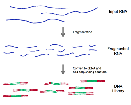
- Record covariates, including processing day -- likely 'batch effects'
3. (Illumina) Sequencing (Bentley et al., 2008,
doi:10.1038/nature07517

- Primary output: FASTQ files of short reads and their [quality
scores](http://en.wikipedia.org/wiki/FASTQ_format#Encoding)
4. Alignment
- Choose to match task, e.g., [Rsubread][], Bowtie2 good for ChIPseq,
some forms of RNAseq; BWA, GMAP better for variant calling
- Primary output: BAM files of aligned reads
5. Reduction
- e.g., RNASeq 'count table' (simple spreadsheets), DNASeq called
variants (VCF files), ChIPSeq peaks (BED, WIG files)
6. Analysis
- Differential expression, peak identification, ...
7. Comprehension
- Biological context

# Sequence data representations
## DNA / amino acid sequences: FASTA files
Input & manipulation: [Biostrings][]
>NM_078863_up_2000_chr2L_16764737_f chr2L:16764737-16766736
gttggtggcccaccagtgccaaaatacacaagaagaagaaacagcatctt
gacactaaaatgcaaaaattgctttgcgtcaatgactcaaaacgaaaatg
...
atgggtatcaagttgccccgtataaaaggcaagtttaccggttgcacggt
>NM_001201794_up_2000_chr2L_8382455_f chr2L:8382455-8384454
ttatttatgtaggcgcccgttcccgcagccaaagcactcagaattccggg
cgtgtagcgcaacgaccatctacaaggcaatattttgatcgcttgttagg
...
Whole genomes: `2bit` and `.fa` formats: [rtracklayer][],
[Rsamtools][]; [BSgenome][]
## Reads: FASTQ files
Input & manipulation: [ShortRead][] `readFastq()`, `FastqStreamer()`,
`FastqSampler()`
@ERR127302.1703 HWI-EAS350_0441:1:1:1460:19184#0/1
CCTGAGTGAAGCTGATCTTGATCTACGAAGAGAGATAGATCTTGATCGTCGAGGAGATGCTGACCTTGACCT
+
HHGHHGHHHHHHHHDGG>CE?=896=:
@ERR127302.1704 HWI-EAS350_0441:1:1:1460:16861#0/1
GCGGTATGCTGGAAGGTGCTCGAATGGAGAGCGCCAGCGCCCCGGCGCTGAGCCGCAGCCTCAGGTCCGCCC
+
DE?DD>ED4>EEE>DE8EEEDE8B?EB<@3;BA79?,881B?@73;1?########################
- Quality scores: 'phred-like', encoded. See
[wikipedia](http://en.wikipedia.org/wiki/FASTQ_format#Encoding)
## Aligned reads: BAM files (e.g., ERR127306_chr14.bam)
Input & manipulation: 'low-level' [Rsamtools][], `scanBam()`,
`BamFile()`; 'high-level' [GenomicAlignments][]
- Header
@HD VN:1.0 SO:coordinate
@SQ SN:chr1 LN:249250621
@SQ SN:chr10 LN:135534747
@SQ SN:chr11 LN:135006516
...
@SQ SN:chrY LN:59373566
@PG ID:TopHat VN:2.0.8b CL:/home/hpages/tophat-2.0.8b.Linux_x86_64/tophat --mate-inner-dist 150 --solexa-quals --max-multihits 5 --no-discordant --no-mixed --coverage-search --microexon-search --library-type fr-unstranded --num-threads 2 --output-dir tophat2_out/ERR127306 /home/hpages/bowtie2-2.1.0/indexes/hg19 fastq/ERR127306_1.fastq fastq/ERR127306_2.fastq
- Alignments: ID, flag, alignment and mate
ERR127306.7941162 403 chr14 19653689 3 72M = 19652348 -1413 ...
ERR127306.22648137 145 chr14 19653692 1 72M = 19650044 -3720 ...
ERR127306.933914 339 chr14 19653707 1 66M120N6M = 19653686 -213 ...
ERR127306.11052450 83 chr14 19653707 3 66M120N6M = 19652348 -1551 ...
ERR127306.24611331 147 chr14 19653708 1 65M120N7M = 19653675 -225 ...
ERR127306.2698854 419 chr14 19653717 0 56M120N16M = 19653935 290 ...
ERR127306.2698854 163 chr14 19653717 0 56M120N16M = 19653935 2019 ...
- Alignments: sequence and quality
... GAATTGATCAGTCTCATCTGAGAGTAACTTTGTACCCATCACTGATTCCTTCTGAGACTGCCTCCACTTCCC *'%%%%%#&&%''#'&%%%)&&%%$%%'%%'&*****$))$)'')'%)))&)%%%%$'%%%%&"))'')%))
... TTGATCAGTCTCATCTGAGAGTAACTTTGTACCCATCACTGATTCCTTCTGAGACTGCCTCCACTTCCCCAG '**)****)*'*&*********('&)****&***(**')))())%)))&)))*')&***********)****
... TGAGAGTAACTTTGTACCCATCACTGATTCCTTCTGAGACTGCCTCCACTTCCCCAGCAGCCTCTGGTTTCT '******&%)&)))&")')'')'*((******&)&'')'))$))'')&))$)**&&****************
... TGAGAGTAACTTTGTACCCATCACTGATTCCTTCTGAGACTGCCTCCACTTCCCCAGCAGCCTCTGGTTTCT ##&&(#')$')'%&&#)%$#$%"%###&!%))'%%''%'))&))#)&%((%())))%)%)))%*********
... GAGAGTAACTTTGTACCCATCACTGATTCCTTCTGAGACTGCCTCCACTTCCCCAGCAGCCTCTGGTTTCTT )&$'$'$%!&&%&&#!'%'))%''&%'&))))''$""'%'%&%'#'%'"!'')#&)))))%$)%)&'"')))
... TTTGTACCCATCACTGATTCCTTCTGAGACTGCCTCCACTTCCCCAGCAGCCTCTGGTTTCTTCATGTGGCT ++++++++++++++++++++++++++++++++++++++*++++++**++++**+**''**+*+*'*)))*)#
... TTTGTACCCATCACTGATTCCTTCTGAGACTGCCTCCACTTCCCCAGCAGCCTCTGGTTTCTTCATGTGGCT ++++++++++++++++++++++++++++++++++++++*++++++**++++**+**''**+*+*'*)))*)#
- Alignments: Tags
... AS:i:0 XN:i:0 XM:i:0 XO:i:0 XG:i:0 NM:i:0 MD:Z:72 YT:Z:UU NH:i:2 CC:Z:chr22 CP:i:16189276 HI:i:0
... AS:i:0 XN:i:0 XM:i:0 XO:i:0 XG:i:0 NM:i:0 MD:Z:72 YT:Z:UU NH:i:3 CC:Z:= CP:i:19921600 HI:i:0
... AS:i:0 XN:i:0 XM:i:0 XO:i:0 XG:i:0 NM:i:4 MD:Z:72 YT:Z:UU XS:A:+ NH:i:3 CC:Z:= CP:i:19921465 HI:i:0
... AS:i:0 XN:i:0 XM:i:0 XO:i:0 XG:i:0 NM:i:4 MD:Z:72 YT:Z:UU XS:A:+ NH:i:2 CC:Z:chr22 CP:i:16189138 HI:i:0
... AS:i:0 XN:i:0 XM:i:0 XO:i:0 XG:i:0 NM:i:5 MD:Z:72 YT:Z:UU XS:A:+ NH:i:3 CC:Z:= CP:i:19921464 HI:i:0
... AS:i:0 XM:i:0 XO:i:0 XG:i:0 MD:Z:72 NM:i:0 XS:A:+ NH:i:5 CC:Z:= CP:i:19653717 HI:i:0
... AS:i:0 XM:i:0 XO:i:0 XG:i:0 MD:Z:72 NM:i:0 XS:A:+ NH:i:5 CC:Z:= CP:i:19921455 HI:i:1
## Called variants: VCF files
Input and manipulation: [VariantAnnotation][] `readVcf()`,
`readInfo()`, `readGeno()` selectively with `ScanVcfParam()`.
- Header
##fileformat=VCFv4.2
##fileDate=20090805
##source=myImputationProgramV3.1
##reference=file:///seq/references/1000GenomesPilot-NCBI36.fasta
##contig=
##phasing=partial
##INFO=
##INFO=
...
##FILTER=
##FILTER=
...
##FORMAT=
##FORMAT=
- Location
#CHROM POS ID REF ALT QUAL FILTER ...
20 14370 rs6054257 G A 29 PASS ...
20 17330 . T A 3 q10 ...
20 1110696 rs6040355 A G,T 67 PASS ...
20 1230237 . T . 47 PASS ...
20 1234567 microsat1 GTC G,GTCT 50 PASS ...
- Variant INFO
#CHROM POS ... INFO ...
20 14370 ... NS=3;DP=14;AF=0.5;DB;H2 ...
20 17330 ... NS=3;DP=11;AF=0.017 ...
20 1110696 ... NS=2;DP=10;AF=0.333,0.667;AA=T;DB ...
20 1230237 ... NS=3;DP=13;AA=T ...
20 1234567 ... NS=3;DP=9;AA=G ...
- Genotype FORMAT and samples
... POS ... FORMAT NA00001 NA00002 NA00003
... 14370 ... GT:GQ:DP:HQ 0|0:48:1:51,51 1|0:48:8:51,51 1/1:43:5:.,.
... 17330 ... GT:GQ:DP:HQ 0|0:49:3:58,50 0|1:3:5:65,3 0/0:41:3
... 1110696 ... GT:GQ:DP:HQ 1|2:21:6:23,27 2|1:2:0:18,2 2/2:35:4
... 1230237 ... GT:GQ:DP:HQ 0|0:54:7:56,60 0|0:48:4:51,51 0/0:61:2
... 1234567 ... GT:GQ:DP 0/1:35:4 0/2:17:2 1/1:40:3
## Genome annotations: BED, WIG, GTF, etc. files
Input: [rtracklayer][] `import()`
- BED: range-based annotation (see
http://genome.ucsc.edu/FAQ/FAQformat.html for definition of this and
related formats)
- WIG / bigWig: dense, continuous-valued data
- GTF: gene model
- Component coordinates
7 protein_coding gene 27221129 27224842 . - . ...
...
7 protein_coding transcript 27221134 27224835 . - . ...
7 protein_coding exon 27224055 27224835 . - . ...
7 protein_coding CDS 27224055 27224763 . - 0 ...
7 protein_coding start_codon 27224761 27224763 . - 0 ...
7 protein_coding exon 27221134 27222647 . - . ...
7 protein_coding CDS 27222418 27222647 . - 2 ...
7 protein_coding stop_codon 27222415 27222417 . - 0 ...
7 protein_coding UTR 27224764 27224835 . - . ...
7 protein_coding UTR 27221134 27222414 . - . ...
- Annotations
gene_id "ENSG00000005073"; gene_name "HOXA11"; gene_source "ensembl_havana"; gene_biotype "protein_coding";
...
... transcript_id "ENST00000006015"; transcript_name "HOXA11-001"; transcript_source "ensembl_havana"; tag "CCDS"; ccds_id "CCDS5411";
... exon_number "1"; exon_id "ENSE00001147062";
... exon_number "1"; protein_id "ENSP00000006015";
... exon_number "1";
... exon_number "2"; exon_id "ENSE00002099557";
... exon_number "2"; protein_id "ENSP00000006015";
... exon_number "2";
...
# R
Language and environment for statistical computing and graphics
- Full-featured programming language
- Interactive and *interpretted* -- convenient and forgiving
- Coherent, extensive documentation
- Statistical, e.g. `factor()`, `NA`
- Extensible -- CRAN, Bioconductor, github, ...
Vector, class, object
- Efficient _vectorized_ calculations on 'atomic' vectors `logical`,
`integer`, `numeric`, `complex`, `character`, `byte`
- Atomic vectors are building blocks for more complicated _objects_
- `matrix` -- atomic vector with 'dim' attribute
- `data.frame` -- list of equal length atomic vectors
- Formal _classes_ represent complicated combinations of vectors,
e.g., the return value of `lm()`, below
Function, generic, method
- Functions transform inputs to outputs, perhaps with side effects,
e.g., `rnorm(1000)`
- Argument matching first by name, then by position
- Functions may define (some) arguments to have default values
- _Generic_ functions dispatch to specific _methods_ based on class of
argument(s), e.g., `print()`.
- Methods are functions that implement specific generics, e.g.,
`print.factor`; methods are invoked _indirectly_, via the generic.
Introspection
- General properties, e.g., `class()`, `str()`
- Class-specific properties, e.g., `dim()`
Help
- `?print`: help on the generic print
- `?print.data.frame`: help on print method for objects of class
data.frame.
Example
```{r}
x <- rnorm(1000) # atomic vectors
y <- x + rnorm(1000, sd=.5)
df <- data.frame(x=x, y=y) # object of class 'data.frame'
plot(y ~ x, df) # generic plot, method plot.formula
fit <- lm(y ~x, df) # object of class 'lm'
methods(class=class(fit)) # introspection
```
# Bioconductor
## Overview
Analysis and comprehension of high-throughput genomic data
- Statistical analysis: large data, technological artifacts, designed
experiments; rigorous
- Comprehension: biological context, visualization, reproducibility
- High-throughput
- Sequencing: RNASeq, ChIPSeq, variants, copy number, ...
- Microarrays: expression, SNP, ...
- Flow cytometry, proteomics, images, ...
Packages, vignettes, work flows
- 934 packages
- Discover and navigate via [biocViews][]
- Package 'landing page'
- Title, author / maintainer, short description, citation,
installation instructions, ..., download statistics
- All user-visible functions have help pages, most with runnable
examples
- 'Vignettes' an important feature in Bioconductor -- narrative
documents illustrating how to use the package, with integrated code
- 'Release' (every six months) and 'devel' branches
- [Support site](https://support.bioconductor.org);
[videos](https://www.youtube.com/user/bioconductor), [recent
courses](http://bioconductor.org/help/course-materials/)
Objects
- Represent complicated data types
- Foster interoperability
- S4 object system
- Introspection: `methods()`, `getClass()`, `selectMethod()`
- 'accessors' and other documented functions / methods for
manipulation, rather than direct access to the object structure
- Interactive help
- `method?"substr,"` to select help on methods, `class?D`
for help on classes
Example
```{r Biostrings, message=FALSE}
require(Biostrings) # Biological sequences
data(phiX174Phage) # sample data, see ?phiX174Phage
phiX174Phage
m <- consensusMatrix(phiX174Phage)[1:4,] # nucl. x position counts
polymorphic <- which(colSums(m != 0) > 1)
m[, polymorphic]
methods(class=class(phiX174Phage))
selectMethod(reverseComplement, class(phiX174Phage))
```

## A sequence analysis package tour
This very open-ended topic points to some of the most prominent
Bioconductor packages for sequence analysis. Use the opportunity in
this lab to explore the package vignettes and help pages highlighted
below; many of the material will be covered in greater detail in
subsequent labs and lectures.
Basics
- Bioconductor packages are listed on the [biocViews][] page. Each
package has 'biocViews' (tags from a controlled vocabulary)
associated with it; these can be searched to identify appropriately
tagged packages, as can the package title and author.
- Each package has a 'landing page', e.g., for
[GenomicRanges][]. Visit this landing page, and note the
description, authors, and installation instructions. Packages are
often written up in the scientific literature, and if available the
corresponding citation is present on the landing page. Also on the
landing page are links to the vignettes and reference manual and, at
the bottom, an indication of cross-platform availability and
download statistics.
- A package needs to be installed once, using the instructions on the
landing page. Once installed, the package can be loaded into an R
session
```{r require}
library(GenomicRanges)
```
and the help system queried interactively, as outlined above:
```{r help, eval=FALSE}
help(package="GenomicRanges")
vignette(package="GenomicRanges")
vignette(package="GenomicRanges", "GenomicRangesHOWTOs")
?GRanges
```
Domain-specific analysis -- explore the landing pages, vignettes, and
reference manuals of two or three of the following packages.
- Important packages for analysis of differential expression include
[edgeR][] and [DESeq2][]; both have excellent vignettes for
exploration. Additional research methods embodied in Bioconductor
packages can be discovered by visiting the [biocViews][] web page,
searching for the 'DifferentialExpression' view term, and narrowing
the selection by searching for 'RNA seq' and similar.
- Popular ChIP-seq packages include [csaw][] an d[DiffBind][] for
comparison of peaks across samples, [ChIPQC][] for quality
assessment, and [ChIPseeker][] for annotating results (e.g.,
discovering nearby genes). What other ChIP-seq packages are listed
on the [biocViews][] page?
- Working with called variants (VCF files) is facilitated by packages
such as [VariantAnnotation][], [VariantFiltering][], [ensemblVEP][],
and [SomaticSignatures][]; packages for calling variants include,
e.g., [h5vc][] and [VariantTools][].
- Several packages identify copy number variants from sequence data,
including [cn.mops][]; from the [biocViews][] page, what other copy
number packages are available? The [CNTools][] package provides some
useful facilities for comparison of segments across samples.
- Microbiome and metagenomic analysis is facilitated by packages such
as [phyloseq][] and [metagenomeSeq][].
- Metabolomics, chemoinformatics, image analysis, and many other
high-throughput analysis domains are also represented in
Bioconductor; explore these via biocViews and title searches.
Working with sequences, alignments, common web file formats, and raw
data; these packages rely very heavily on the [IRanges][] /
[GenomicRanges][] infrastructure that we will encounter later in the
course.
- The [Biostrings][] package is used to represent DNA and other
sequences, with many convenient sequence-related functions. Check
out the functions documented on the help page `?consensusMatrix`,
for instance. Also check out the [BSgenome][] package for working
with whole genome sequences, e.g., `?"getSeq,BSgenome-method"`
- The [GenomicAlignments][] package is used to input reads aligned to
a reference genome. See for instance the `?readGAlignments` help
page and `vigentte(package="GenomicAlignments",
"summarizeOverlaps")`
- [rtracklayer][]'s `import` and `export` functions can read in many
common file types, e.g., BED, WIG, GTF, ..., in addition to querying
and navigating the UCSC genome browser. Check out the `?import` page
for basic usage.
- The [ShortRead][] and [Rsamtools][] packages can be used for
lower-level access to FASTQ and BAM files, respectively. Explore the
[ShortRead vignette](http://bioconductor.org/packages/release/bioc/vignettes/ShortRead/inst/doc/Overview.pdf)
and Scalable Genomics labs to see approaches to effectively
processing the large files.
Visualization
- The [Gviz][] package provides great tools for visualizing local
genomic coordinates and associated data.
- [epivizr][] drives the [epiviz](http://epiviz.cbcb.umd.edu/) genome
browser from within R; [rtracklayer][] provides easy ways to
transfer data to and manipulate UCSC browser sessions.
- Additionl packages include [ggbio][], [OmicCircos][], ...
## DNA or amino acid sequences: _Biostrings_, _ShortRead_, _BSgenome_
Classes
- XString, XStringSet, e.g., DNAString (genomes),
DNAStringSet (reads)
Methods --
- [Cheat sheat](http://bioconductor.org/packages/release/bioc/vignettes/Biostrings/inst/doc/BiostringsQuickOverview.pdf)
- Manipulation, e.g., `reverseComplement()`
- Summary, e.g., `letterFrequency()`
- Matching, e.g., `matchPDict()`, `matchPWM()`
Related packages
- [BSgenome][]
- Whole-genome representations
- Model and custom
- [ShortRead][]
- FASTQ files
Example
- Whole-genome sequences are distrubuted by ENSEMBL, NCBI, and others
as FASTA files; model organism whole genome sequences are packaged
into more user-friendly `BSgenome` packages. The following
calculates GC content across chr14.
```{r BSgenome-require, message=FALSE}
require(BSgenome.Hsapiens.UCSC.hg19)
chr14_range = GRanges("chr14", IRanges(1, seqlengths(Hsapiens)["chr14"]))
chr14_dna <- getSeq(Hsapiens, chr14_range)
letterFrequency(chr14_dna, "GC", as.prob=TRUE)
```
## Ranges: _GenomicRanges_, _IRanges_
Ranges represent:
- Data, e.g., aligned reads, ChIP peaks, SNPs, CpG islands, ...
- Annotations, e.g., gene models, regulatory elements, methylated
regions
- Ranges are defined by chromosome, start, end, and strand
- Often, metadata is associated with each range, e.g., quality of
alignment, strength of ChIP peak
Many common biological questions are range-based
- What reads overlap genes?
- What genes are ChIP peaks nearest?
- ...
The [GenomicRanges][] package defines essential classes and methods
- `GRanges`

- `GRangesList`

### Range operations

Ranges
- IRanges
- `start()` / `end()` / `width()`
- List-like -- `length()`, subset, etc.
- 'metadata', `mcols()`
- GRanges
- 'seqnames' (chromosome), 'strand'
- `Seqinfo`, including `seqlevels` and `seqlengths`
Intra-range methods
- Independent of other ranges in the same object
- GRanges variants strand-aware
- `shift()`, `narrow()`, `flank()`, `promoters()`, `resize()`,
`restrict()`, `trim()`
- See `?"intra-range-methods"`
Inter-range methods
- Depends on other ranges in the same object
- `range()`, `reduce()`, `gaps()`, `disjoin()`
- `coverage()` (!)
- see `?"inter-range-methods"`
Between-range methods
- Functions of two (or more) range objects
- `findOverlaps()`, `countOverlaps()`, ..., `%over%`, `%within%`,
`%outside%`; `union()`, `intersect()`, `setdiff()`, `punion()`,
`pintersect()`, `psetdiff()`
Example
```{r ranges, message=FALSE}
require(GenomicRanges)
gr <- GRanges("A", IRanges(c(10, 20, 22), width=5), "+")
shift(gr, 1) # 1-based coordinates!
range(gr) # intra-range
reduce(gr) # inter-range
coverage(gr)
setdiff(range(gr), gr) # 'introns'
```
IRangesList, GRangesList
- List: all elements of the same type
- Many *List-aware methods, but a common 'trick': apply a vectorized
function to the unlisted representaion, then re-list
grl <- GRangesList(...)
orig_gr <- unlist(grl)
transformed_gr <- FUN(orig)
transformed_grl <- relist(, grl)
Reference
- Lawrence M, Huber W, Pagès H, Aboyoun P, Carlson M, et al. (2013)
Software for Computing and Annotating Genomic Ranges. PLoS Comput
Biol 9(8): e1003118. doi:10.1371/journal.pcbi.1003118
## Aligned reads: _GenomicAlignments_, _Rsamtools_
Classes -- GenomicRanges-like behaivor
- GAlignments, GAlignmentPairs, GAlignmentsList
- SummarizedExperiment
- Matrix where rows are indexed by genomic ranges, columns by a
DataFrame.
Methods
- `readGAlignments()`, `readGAlignmentsList()`
- Easy to restrict input, iterate in chunks
- `summarizeOverlaps()`
Example
- Find reads supporting the junction identified above, at position
19653707 + 66M = 19653773 of chromosome 14
```{r bam-require}
require(GenomicRanges)
require(GenomicAlignments)
require(Rsamtools)
## our 'region of interest'
roi <- GRanges("chr14", IRanges(19653773, width=1))
## sample data
require('RNAseqData.HNRNPC.bam.chr14')
bf <- BamFile(RNAseqData.HNRNPC.bam.chr14_BAMFILES[[1]], asMates=TRUE)
## alignments, junctions, overlapping our roi
paln <- readGAlignmentsList(bf)
j <- summarizeJunctions(paln, with.revmap=TRUE)
j_overlap <- j[j %over% roi]
## supporting reads
paln[j_overlap$revmap[[1]]]
```
## Called variants: _VariantAnnotation_, _VariantFiltering_
Classes -- GenomicRanges-like behavior
- VCF -- 'wide'
- VRanges -- 'tall'
Functions and methods
- I/O and filtering: `readVcf()`, `readGeno()`, `readInfo()`,
`readGT()`, `writeVcf()`, `filterVcf()`
- Annotation: `locateVariants()` (variants overlapping ranges),
`predictCoding()`, `summarizeVariants()`
- SNPs: `genotypeToSnpMatrix()`, `snpSummary()`
Example
- Read variants from a VCF file, and annotate with respect to a known
gene model
```{r vcf, message=FALSE}
## input variants
require(VariantAnnotation)
fl <- system.file("extdata", "chr22.vcf.gz", package="VariantAnnotation")
vcf <- readVcf(fl, "hg19")
seqlevels(vcf) <- "chr22"
## known gene model
require(TxDb.Hsapiens.UCSC.hg19.knownGene)
coding <- locateVariants(rowRanges(vcf),
TxDb.Hsapiens.UCSC.hg19.knownGene,
CodingVariants())
head(coding)
```
Related packages
- [ensemblVEP][]
- Forward variants to Ensembl Variant Effect Predictor
- [VariantTools][], [h5vc][]
- Call variants
- [VariantFiltering][]
- Filter variants using criteria such as coding consequence, MAF,
..., inheritance model
Reference
- Obenchain, V, Lawrence, M, Carey, V, Gogarten, S, Shannon, P, and
Morgan, M. VariantAnnotation: a Bioconductor package for exploration
and annotation of genetic variants. Bioinformatics, first published
online March 28, 2014
[doi:10.1093/bioinformatics/btu168](http://bioinformatics.oxfordjournals.org/content/early/2014/04/21/bioinformatics.btu168)
## Integrated data representations: _SummarizedExperiment_

[SummarizedExperiment][]
- 'feature' x 'sample' `assays()`
- `colData()` data frame for desciption of samples
- `rowRanges()` _GRanges_ / _GRangeList_ or data frame for description
of features
- `exptData()` to describe the entire object
```{r SummarizedExperiment}
library(SummarizedExperiment)
library(airway)
data(airway)
airway
colData(airway)
airway[, airway$dex %in% "trt"]
```
## Annotation: _org_, _TxDb_, _AnnotationHub_, _biomaRt_, ...
- _Bioconductor_ provides extensive access to 'annotation' resources
(see the [AnnotationData][] biocViews hierarchy); some interesting
examples to explore during this lab include:
- [biomaRt][], [PSICQUIC][], [KEGGREST][] and other packages for
querying on-line resources; each of these have informative vignettes.
- [AnnotationDbi][] is a cornerstone of the
[Annotation Data][AnnotationData] packages provided by Bioconductor.
- **org** packages (e.g., [org.Hs.eg.db][]) contain maps between
different gene identifiers, e.g., ENTREZ and SYMBOL. The basic
interface to these packages is described on the help page `?select`
- **TxDb** packages (e.g., [TxDb.Hsapiens.UCSC.hg19.knownGene][])
contain gene models (exon coordinates, exon / transcript
relationships, etc) derived from common sources such as the hg19
knownGene track of the UCSC genome browser. These packages can be
queried, e.g., as described on the `?exonsBy` page to retrieve all
exons grouped by gene or transcript.
- **BSgenome** packages (e.g., [BSgenome.Hsapiens.UCSC.hg19][])
contain whole genomes of model organisms.
- [VariantAnnotation][] and [ensemblVEP][] provide access to sequence
annotation facilities, e.g., to identify coding variants; see the
[Introduction to VariantAnnotation](http://bioconductor.org/packages/release/bioc/vignettes/ShortRead/inst/doc/Overview.pdf)
vignette for a brief introduction.
- Take a quick look at the [annotation work
flow](http://bioconductor.org/help/workflows/annotation/annotation/)
on the Bioconductor web site.
## Scalable computing
1. Efficient _R_ code
- Vectorize!
- Reuse others' work Know -- [DESeq2][], [GenomicRanges][],
[Biostrings][], [dplyr][], [data.table][], [Rcpp][]
2. Iteration
- Chunk-wise
- `open()`, read chunk(s), `close()`.
- e.g., `yieldSize` argument to `Rsamtools::BamFile()`
3. Restriction
- Limit to columns and / or rows of interest
- Exploit domain-specific formats, e.g., BAM files and
`Rsamtools::ScanBamParam()`
- Use a data base
4. Sampling
- Iterate through large data, retaining a manageable sample, e.g.,
`ShortRead::FastqSampler()`
5. Parallel evaluation
- **After** writing efficient code
- Typically, `lapply()`-like operations
- Cores on a single machine ('easy'); clusters (more tedious);
clouds
Parallel evaluation in _Bioconductor_
- [BiocParallel][] -- `bplapply()` for `lapply()`-like functions,
increasingly used by package developers to provide easy, standard
way of gaining parallel evaluation.
- [GenomicFiles][] -- Framework for working on groups of files,
ranges, or ranges x files
- Bioconductor [AMI][] (Amazon Machine Instance) including
pre-configured StarCluster, and [docker] containers�.
# Resources
_R_ / _Bioconductor_
- [Web site][Bioconductor] -- install, learn, use, develop _R_ /
_Bioconductor_ packages
- [Support](http://support.bioconductor.org) -- seek help and
guidance; also
[StackOverflow](http://stackoverflow.com/questions/tagged/r) for _R_
programming questions
- [biocViews](http://bioconductor.org/packages/release/BiocViews.html)
-- discover packages
- Package landing pages, e.g.,
[GenomicRanges](http://bioconductor.org/packages/release/bioc/html/GenomicRanges.html),
including title, description, authors, installation instructions,
vignettes (e.g., GenomicRanges '[How
To](http://bioconductor.org/packages/release/bioc/vignettes/GenomicRanges/inst/doc/GenomicRangesHOWTOs.pdf)'),
etc.
- [Course](http://bioconductor.org/help/course-materials/) and other
[help](http://bioconductor.org/help/) material (e.g., videos, EdX
course, community blogs, ...)
Publications (General _Bioconductor_)
- Lawrence M, Huber W, Pagès H, Aboyoun P, Carlson M, et al. (2013)
Software for Computing and Annotating Genomic Ranges. PLoS Comput
Biol 9(8): e1003118. doi:
[10.1371/journal.pcbi.1003118][GRanges.bib]
- Lawrence, M, and Morgan, M. 2014. Scalable Genomics with R and
Bioconductor. Statistical Science 2014, Vol. 29, No. 2,
214-226. [http://arxiv.org/abs/1409.2864v1][Scalable.bib]
Other
- Lawrence, M. 2014. Software for Enabling Genomic Data
Analysis. Bioc2014 conference [slides][Lawrence.bioc2014.bib].
[R]: http://r-project.org
[Bioconductor]: http://bioconductor.org
[GRanges.bib]: http://dx.doi.org/10.1371/journal.pcbi.1003118
[Scalable.bib]: http://arxiv.org/abs/1409.2864
[Lawrence.bioc2014.bib]:
http://bioconductor.org/help/course-materials/2014/BioC2014/Lawrence_Talk.pdf
[AnnotationData]: http://bioconductor.org/packages/release/BiocViews.html#___AnnotationData
[biocViews]: http://bioconductor.org/packages/release/BiocViews.html#___Software
[AnnotationDbi]: http://bioconductor.org/packages/AnnotationDbi
[AnnotationHub]: http://bioconductor.org/packages/AnnotationHub
[BSgenome.Hsapiens.UCSC.hg19]: http://bioconductor.org/packages/BSgenome.Hsapiens.UCSC.hg19
[BSgenome]: http://bioconductor.org/packages/BSgenome
[BiocParallel]: http://bioconductor.org/packages/BiocParallel
[Biostrings]: http://bioconductor.org/packages/Biostrings
[CNTools]: http://bioconductor.org/packages/CNTools
[ChIPQC]: http://bioconductor.org/packages/ChIPQC
[ChIPseeker]: http://bioconductor.org/packages/ChIPseeker
[DESeq2]: http://bioconductor.org/packages/DESeq2
[DiffBind]: http://bioconductor.org/packages/DiffBind
[GenomicAlignments]: http://bioconductor.org/packages/GenomicAlignments
[GenomicFiles]: http://bioconductor.org/packages/GenomicFiles
[GenomicRanges]: http://bioconductor.org/packages/GenomicRanges
[Homo.sapiens]: http://bioconductor.org/packages/Homo.sapiens
[IRanges]: http://bioconductor.org/packages/IRanges
[KEGGREST]: http://bioconductor.org/packages/KEGGREST
[PSICQUIC]: http://bioconductor.org/packages/PSICQUIC
[Rsamtools]: http://bioconductor.org/packages/Rsamtools
[Rsubread]: http://bioconductor.org/packages/Rsubread
[ShortRead]: http://bioconductor.org/packages/ShortRead
[SomaticSignatures]: http://bioconductor.org/packages/SomaticSignatures
[SummarizedExperiment]: http://bioconductor.org/packages/SummarizedExperiment
[TxDb.Hsapiens.UCSC.hg19.knownGene]: http://bioconductor.org/packages/TxDb.Hsapiens.UCSC.hg19.knownGene
[VariantAnnotation]: http://bioconductor.org/packages/VariantAnnotation
[VariantFiltering]: http://bioconductor.org/packages/VariantFiltering
[VariantTools]: http://bioconductor.org/packages/VariantTools
[biomaRt]: http://bioconductor.org/packages/biomaRt
[cn.mops]: http://bioconductor.org/packages/cn.mops
[csaw]: http://bioconductor.org/packages/csaw
[edgeR]: http://bioconductor.org/packages/edgeR
[ensemblVEP]: http://bioconductor.org/packages/ensemblVEP
[h5vc]: http://bioconductor.org/packages/h5vc
[limma]: http://bioconductor.org/packages/limma
[metagenomeSeq]: http://bioconductor.org/packages/metagenomeSeq
[org.Hs.eg.db]: http://bioconductor.org/packages/org.Hs.eg.db
[org.Sc.sgd.db]: http://bioconductor.org/packages/org.Sc.sgd.db
[phyloseq]: http://bioconductor.org/packages/phyloseq
[rtracklayer]: http://bioconductor.org/packages/rtracklayer
[snpStats]: http://bioconductor.org/packages/snpStats
[Gviz]: http://bioconductor.org/packages/Gviz
[epivizr]: http://bioconductor.org/packages/epivizr
[ggbio]: http://bioconductor.org/packages/ggbio
[OmicCircos]: http://bioconductor.org/packages/OmicCircos
[dplyr]: https://cran.r-project.org/package=dplyr
[data.table]: https://cran.r-project.org/package=data.table
[Rcpp]: https://cran.r-project.org/package=Rcpp
[AMI]: http://bioconductor.org/help/bioconductor-cloud-ami/
[docker]: http://bioconductor.org/help/docker/